Sweep
VEP (Visual Evoked Potential)
Ai-Hou
Wang, M.D., Ph.D.
��1990�L��1991�L�b�ª��sThe Smith-Kettlewell Eye Research Institute (SKERI)�i�פp���α�(Fellowship of Pediatric Ophthalmology and Strabismus)���@�~���A������IJ���M�q�Ͳz���]�p�A��@�ODr. Erich Sutter���h�J�����q��(Multifocal ERG)�A��G�ODr. Anthony Norcia�MDr. Christopher Tyler�����������o�q��(Sweep VEP)�C�ثe����{�ɵ�ı�q�Ͳz�Ƿ|(International Society for
Clinical Electrophysiology of Vision, ISCEV)�w�g���h�J�����q�Ϫ��з�(https://iscev.wildapricot.org/standards)�A���������o�q�쪺�з��٨S���C�J�C���F�{�ɨϥΤ��~�A�o�ⶵ�u��]�O��ı����¦��Ǭ�s���Q���C
During my year-long Fellowship of Pediatric Ophthalmology and
Strabismus at The Smith-Kettlewell Eye Research Institute (SKERI) in San
Francisco from the summer of 1990 to the summer of 1991, I had the opportunity
to learn about two electrophysiological designs: Dr. Erich Sutter's multifocal
electroretinography (ERG) and Dr. Anthony Norcia and Dr. Christopher Tyler's
sweep visual evoked potentials (Sweep VEP). Currently, the International
Society for Clinical Electrophysiology of Vision (ISCEV) has standards for
multifocal ERG (https://iscev.wildapricot.org/standards), but standards for sweep visual evoked potentials have not yet been included.
Besides clinical use, these two tools are also invaluable for basic scientific
research in vision.


Dr. Anthony Norcia Dr. Christopher Tyler
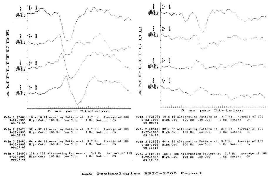
�{�ɤW�Ϲ������o�q��(Pattern
Visual Evoked Potential)�ϥΦ�v�ѽL����(Checkerboard
reversal)�A�Ⲵ���}�U�ۧ@�A�C�@���@�|���j�p����l
�V �C��16��A32��A64��M128��(����)�A��l���j�p�h�O���1�X�A1/2�X�A1/4�X�M1/8�X�C�Y�Ԫ�����ǨC�ر��ҧ@�⦸�A�N�i�����|�@�_�A�i�ܹ��窺í�w�ʩM�i���{��(Reproducibility)�C
Clinically,
pattern visual evoked potentials (PDPs) are performed using checkerboard
reversal, with each eye tested separately. Each eye tests four different grid
sizes �V 16, 32, 64, and 128 squares per side (see figure), with grid sizes of
1�X, 1/2�X, 1/4�X, and 1/8�X. In rigorous laboratory settings, each scenario is
tested twice, with the waveforms superimposed to demonstrate the stability and
reproducibility of the experiment.


�q�`�@�ȺA�����o�q��(Transient
VEP)�A�C������3.7��(3.7reversals)(����)�C�[�`100�����i(average)�H�����T����(Signal/Noise Ratio)��100=10���C�ܤֻݮ�27��(3.7
reversals/sec à
27 sec/100reversals)�C������q�`�S����k���ɶ��`���۳o��L�᪺�e���C
�o�O�@�쥪���z�����f�H�A�k�����O���ΡA1/8�X�̤p����l���M���o�X�j�q��A��l���p�A�i���p������v���Ԫ��C�����z���A�ĤG���B1/2�X��l�����o�q��w�g�ݤ��MNPN�i���F�C
Transient
visual evoked potentials (VEPs) are typically performed, with 3.7 reversals per
second (see figure). The average of 100 brainwaves is summed to improve the
signal-to-noise ratio (SNR) by ��100 = 10 times. This
requires at least 27 seconds (3.7 reversals/sec ��
27 sec/100 reversals). Infants and young children typically cannot stare at
such a boring image for an extended period.
This
is a patient with amblyopia in the left eye and excellent vision in the right
eye. Even the smallest square at 1/8�X still evoked a large potential; as the
squares decreased, the peak-to-trough potentials
gradually lengthened. In the left eye with amblyopia, the NPN waveform in the
second square at 1/2�X was no longer clearly visible.
���F�H�q�Ͳz����k�ֳt������ı�\��A�b1970�B1980�~�N�ADr. Christopher Tyler�MDr. Anthony Norcia�}�o�F���������o�q��(Sweep VEP)���t���A���p�p����O(visual acuity)�B���ӷP��(contrast
sensitivity)�M��е��O(vernier acuity)���o�|�C�o�Өt�Υ�1970�B80�~�N�o�i�ܤ��A�s��PowerDiva�C
To rapidly assess visual function using electrophysiological
methods, Dr. Christopher Tyler and Dr. Anthony Norcia developed the sweep
visual evoked potential (SEP) system in the 1970s and 1980s to estimate the
development of visual acuity, contrast sensitivity, and vernier acuity in
children. This system, developed from the 1970s and 80s to the present day, is
called PowerDiva.
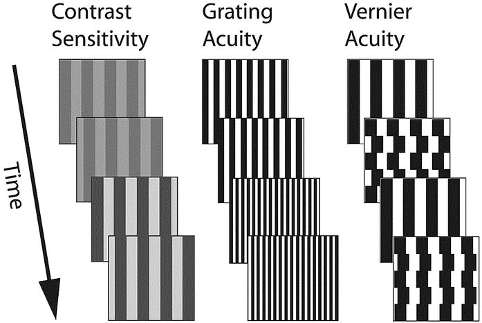
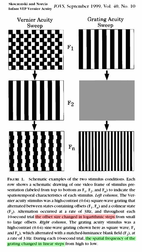
�u�n�O��10�������i�C�@í�A�����o�q��A�C�b���ܴ��@���Ϲ����ѼơA10���@�i��20�ؤj�p�C
�������O�A�O�������]���A���e�ӯ��A�̪Ŷ��W�v(spatial
frequency)�u��(linear)�a����20���e��(����)�C
Only 10 seconds of brainwave recording are
needed. Steady-state visual evoked potentials are generated, with image
parameters changing every half second, displaying 20 different sizes over 10
seconds.
Visual acuity is assessed using a sinusoidal
grating, sweeping across 20 widths linearly according to spatial frequency,
from wide to narrow (see figure).
Sweep Spatial Frequecy (Size) (Visual
Acuity)
Linearly from Low to High Spatial Frequency (From Large to Small
size)

�������ӷP���A�O�ΩT�w�e�ת������]���A��p�Ӥj�A�̹��(contrast)����(logarithmic)�a����20�����(����)�C
To assess contrast sensitivity, a sinusoidal grating of fixed
width was used, with contrasts ranging from small to large, sweeping across 20
contrasts in logarithmic proportions (see figure).
Sweep Contrast (Contrast Sensitivity)
Logarithmically from Low to High Contrast

������е��O�A�O����i�]���A����(offset)�ѯ����e�A�̪Ŷ��W�v(spatial frequency)����(logarithmic)�a����20���e��(����)�C
To assess vernier vision, a square wave grating is used, with
offsets ranging from narrow to wide, sweeping across 20 different widths in
logarithmic proportions according to spatial frequency (see figure).
Sweep Offset (Vernier Acuity)
Logarithmically from Small to Large Offset

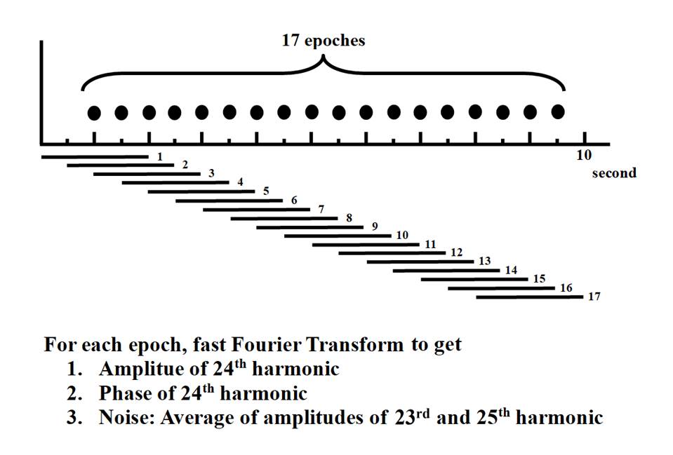
����10�������i�A��2�����@�Ӱ϶� �V 0��2�����@�Ӱ϶��B0.5��2.5�����@�Ӱ϶��B1��3�����@�Ӱ϶��K�K7.5��9.5�����@�Ӱ϶��B8��10�����@�Ӱ϶��A�@�@17�Ӱ϶��C�������O���]���p�G�H6Hz(12 reversals/sec)����A2�����϶��̦�24�Ӥ���A����o2�����i��24���W(24th harmonic)�����T(amplitude)�M�ۦ�(phase)�C�P�ɩ���C�@�϶�23���W(23rd harmonic)�M25���W(25th harmonic)�����T�A��̪������ȷ��@���T(noise)�A���T���C�A����24���W�W�T��O���o�ӨӪ��q��(����)�C
The entire 10-second brainwave was divided into 2-second blocks �V
0 to 2 seconds, 0.5 to 2.5 seconds, 1 to 3 seconds, ... 7.5 to 9.5 seconds, 8
to 10 seconds, for a total of 17 blocks. If the visual acuity grating reverses
at 6 Hz (12 reversals/sec), there are 24 reversals in a 2-second block. The
amplitude and phase of the 24th harmonic of this 2-second brainwave were
extracted. Simultaneously, the amplitudes of the 23rd and 25th harmonics were
extracted from each block, and the average of these two was taken as noise. A
low signal-to-noise ratio indicates that the potential at the 24th harmonic was
indeed induced (see figure).
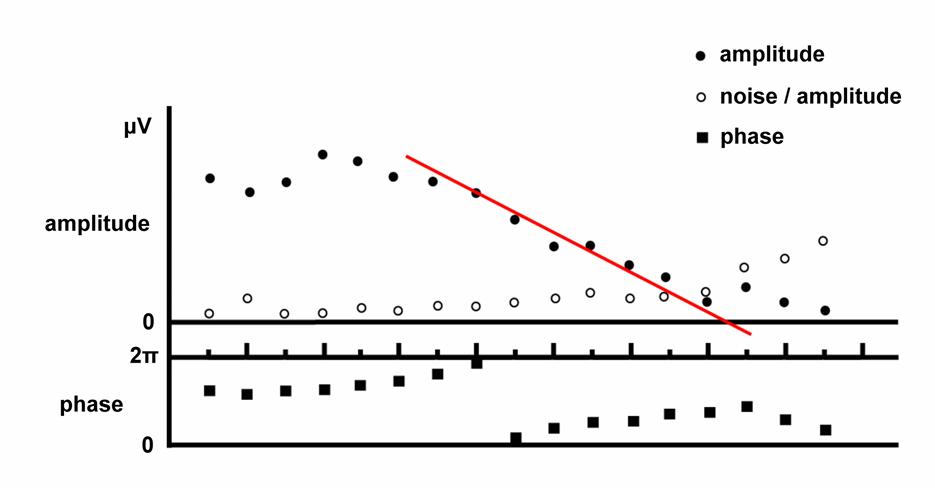
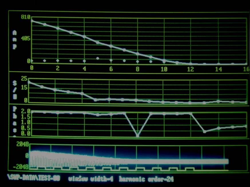
�N17��2���϶��o�쪺17�Ӯ��T�M17�Ӭۦ�A�H��17�Ӱ϶������T�@�Ϧp�U(����)�C������]�������ܯ��A���o�q��T�����ܤp�A�ۦ캥������(�۷���ȺA�����o�q������Ⱥ����ܪ�)�C��X�T�ӭȨӦ��p���O���H��(threshold)�A�]�N�O���p�]���ܨ�h���A���ժ̴N�ݤ������F�C
1. �~��(extrapolate)���Ŷ��W�v�B�����T(���u)�A0�q��B���Ŷ��W�v�@�����O���p�ȡC
2. �ۦ���������A�����Ͷ���V���ܶáA�ӳB���Ŷ��W�v�@�����O���p�ȡC
3. ���T��(noise/signal)�����ܤj�A����ֳt�ܤj���a�誺�Ŷ��W�v�@�����O���p�ȡC(����)
The following diagram plots the 17 amplitudes and 17 phases
obtained from 17 2-second blocks, along with the noise from each block (see
figure). As the inversion grating gradually narrows, the evoked potential
amplitude gradually decreases, and the phase gradually shifts (equivalent to
the potential value of the transient visual evoked potential gradually
increasing). These three values are combined to estimate the visual acuity
threshold, that is, how fine the grating needs to become before the subject can
no longer see the inversion.
1. Extrapolate the amplitude at high spatial frequencies (red
line); the spatial frequency at 0 potential is used as the visual acuity
estimate.
2. Gradually shift the phase; if the shift trend reverses or
becomes disordered, the spatial frequency at that point is used as the visual
acuity estimate.
3. Gradually increase the noise/signal
ratio; the spatial frequency at the point where it increases significantly and
rapidly is used as the visual acuity estimate. (See figure)
�o�M�t�Υi�H���ܪ��ѼƦ��\�h�A���R��k�D�n�ϥγť߸��ഫ����Y�X���W�v�����T�M�ۦ�A�Pı�W�ä����g�C
�q�`�Q�n���D��Y�@�Ѽƪ���ı�H��(Threshold)�A�o�M�t�Ϊ��зdz]�w�O�A����E���ϧΨC�b�����ܤ@���A10�����@����20���ϧΡC�i�H�q����ݱo�M�������ܨ����ݤ��M���A�o�M�t�α������O�A�Ϊ̻��O�Ŷ��W�v(spatial frequency)�A�N�O�Ѥj���������V�p�����F�]�i�H�ۤϹL�ӡA�o�M�t�α������(contrast)�M����������O(vernier acuity)�A�N�O�q����ݤ��M����������������ݱo�M��(����)�C
20�ӹϧΧ��ܪ��覡�M�t�פ]�n�Ҷq�G�������O�ϥ����]�����Ŷ��W�v�O�u��(linear)�ܤƪ��A�Ŷ��W�v�����O�C�����X�P(cycles
per degree)�A�O�������˼ơA�۷���Snellen���O�A�M�{���ϥΪ����(logMAR)���O���N���@�ˤF�C��������A�Ѯz����j���A�C�@�B�O�̹��(logarithmic)�W�[���C����q�`�O��(�̰��G��-�̧C�G��)/�����G���C����������O�A���M�M�]��(grating)���O�@�ˡA�]�O�Ŷ��j�p�������A���O����]���������Ѥp�Ӥj�o�O�̹�ƼW�[��(����)�C
This system allows for the modification of
many parameters. The analysis method primarily uses Fourier transform to
extract the amplitude and phase of certain frequencies, which seems
straightforward to implement.
To determine the visual threshold for a
specific parameter, the standard setting of this system is to change the visual
stimulus pattern every half second, scanning 20 patterns in 10 seconds. The
pattern can gradually transition from relatively clear to relatively unclear;
this system scans for visual acuity, or spatial frequency, moving from large
stripes to small stripes. Conversely, it can scan for contrast and vernier
acuity, gradually transitioning from relatively unclear to relatively clear
(see figure).
The manner and speed of change of the 20
patterns must also be considered: the spatial frequency of the grating used for
visual acuity scanning changes linearly. The unit of spatial frequency is
cycles per degree of visual field (FIN), which is the reciprocal of the FIN,
equivalent to Snellen visual acuity, unlike the logMAR visual acuity charts
used today. Sweeping contrast, from weak to strong, increases logarithmically
at each step. The unit of contrast is usually (highest brightness - lowest
brightness) / average brightness. Sweeping vernier vision, although similar to
grating vision in that it is a concept of spatial size, involves the vernier
grating misalignment increasing logarithmically from small to large (see
figure).
Tyler CW, Apkarian P, Levi DM, Nakayama K.
Rapid assessment of visual function: an electronic sweep technique for the
pattern visual evoked potential. Invest Ophthalmol Vis Sci. 1979
Jul;18(7):703-13.
Norcia
AM, Tyler CW, Hamer RD. Development of contrast sensitivity in the
human infant. Vision Res. 1990;30(10):1475-86.
Skoczenski AM, Norcia AM. Development of VEP
Vernier Acuity and Grating Acuity in Human Infants. Invest Ophthalmol Vis Sci. 1999;40:2411�V2417.
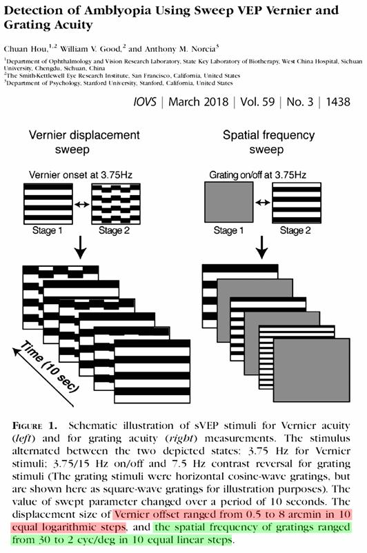
Hou C, Good WV, Norcia AM. Detection of amblyopia
using sweep VEP Vernier and grating acuity. Invest Ophthalmol
Vis Sci. 2018;59:1435�V1442.
�e���ҭz�ť߸����R�O��2�����@�϶��A�۾F�϶����j0.5���A�h10���@��17�Ӱ϶��C���O�p�U�ϡA�p�G���R���϶���1���A���j0.5���A�h10���̴N�|��19���϶��F�C�϶������שM�۾F�϶������j�i�H���N���ܡA�P�ɤ]�M�w�F10���̰϶����`�ơC�Ҧp�϶���3���B�϶����j1���A�h�϶��`�ƬO8�Ӱ϶��C
The Fourier analysis described earlier uses a
2-second block size with a 0.5-second interval between adjacent blocks,
resulting in 17 blocks in 10 seconds. However, as shown in the diagram, if the
analyzed blocks are 1 second long with a 0.5-second interval, there will be 19
blocks in 10 seconds. The block length and the interval between adjacent blocks
can be arbitrarily changed, which also determines the total number of blocks in
10 seconds. For example, if the block length is 3 seconds and the block interval
is 1 second, the total number of blocks is 8.
�p�G����E���W�v�O3.75Hz�A�϶���2���A�h2���̦�7.5�өP���C�ť߸����R7.5���W(7.5th harmonic)�O���W(
�p�G10���������ܹϧΡA���M�N���s�@���������o�q��A���O���¥i�H�Q�γo�Өt�Ϊ��ť߸����R�C�N�쥻2�����϶��Ԫ���10���A���M���{�]�N�u��1�Ӱ϶��C�N�p�Pí�A/�ȺA�����o�q�� Steady-state vs. Transient VEP�@��̴y�z�����B��ı/���ʲ��_������������������o�q�����A����(jittering)���]���p�G�H6Hz�����A10�����`�@���ʤF60�өP���C�b10�������i���A�H�ť߸����R���60���W(60th
harmonic)�����T�M�ۦ��O���W(
If the visual stimulus frequency is 3.75 Hz and the block length is 2
seconds, then there are 7.5 cycles in 2 seconds. Fourier analysis shows that
the 7.5th harmonic is the fundamental frequency (1f), and the 15th harmonic is
the second harmonic (2f).
If the pattern doesn't change for 10 seconds, it's not called a swept
visual evoked potential, but Fourier analysis of this system can still be used.
Extending the original 2-second block to 10 seconds results in only one block
throughout. Similar to the "kinesthetic/optico-nystagmus nasotemporal
asymmetric visual evoked potential" described in the article
"Steady-state vs. Transient VEP," if the jittering grating vibrates
at 6 Hz, it vibrates for a total of 60 cycles in 10 seconds. In a 10-second
brainwave, the amplitude and phase of the 60th harmonic frequency extracted by
Fourier analysis are the fundamental frequency (1f), and the amplitude and
phase of the 120th harmonic frequency are the 2nd harmonic frequency (2f).
����Ϲ�����E���A�j�����q���ù����t��(frame
rate)�C���i�ܤj��60�i�϶H�A�λ�60��(frames)�C�ֳt���϶H�ഫ�A�p�G����b�U�@��/�U�@��X�{���e�����p��B���X�s�e���A�b�q���ù����i�ܥ\��W�A�N��F�����Y����(real-time)�����e�C
�Ϲ������o�q��H�q���ù��e�{�϶H�A�C���e�{60�i�϶H�A�n�������q�v�C���e�{24�i�϶H�@�ˡC�b�϶H1/�϶H2����e�{�����p(�Ҧp��v�ѽL����O��v�ѽL1�M��v�ѽL2����e�{)�A�p�G�C�@�϶H���d1��A�C�@�P�N�O2��A�C���N�O30�P(cycle�AHz)��60����(reversal)�C�p�G�C�@�϶H���d4��A�N�O7.5Hz�B15����F�C�@�϶H���d3��A�N�O10Hz�B20�����K�K�C�`���A�������O��ơB60���o�ɪ���ơC
�@��ı����ɡA3Hz�B6����`�Q�Χ@�C���ɶ��W�v(low temporal frequency)�A��5Hz�B10����`�Q�Χ@�֪��ɶ��W�v(high temporal frequency)�C�ť߸����R������W(
�p�G�q���{���]�p�e�{�϶H���M�ù��P�B�A�Ϊ̨C���϶H�Ƥ��O60�����ơA�ù��W���ʺA�϶H�N�|�X�{�_�u�A�Ө��ժ̱����쪺��ı��E�N���b�A�]�p�B����d���C
Regarding visual evoked potentials (VAPs),
most computer screens display approximately 60 images per second, or 60 frames.
Rapid image transitions, where calculations are completed and new images are
displayed before the next frame appears, represent a "real-time"
threshold in computer screen display functionality.
Visual evoked potentials (VAPs) display
images on a computer screen at 60 frames per second, similar to the 24 frames
per second of film. In cases where image 1/image 2 alternates (e.g., in
chessboard reversal, chessboard 1 and chessboard 2 alternate), if each image
stays on one frame, each cycle is 2 frames, resulting in 30 cycles (Hz) or 60
reversals per second. If each image stays on four frames, it's 7.5 Hz with 15
reversals; if each image stays on three frames, it's 10 Hz with 20 reversals,
and so on. In short, the frequency must be an integer, divisible by 60.
In visual experiments, 3Hz and 6Hz inversion
are often used as low temporal frequencies, while 5Hz and 10Hz inversion are
often used as high temporal frequencies. Fourier analysis extracts the
fundamental frequency (1f) by extracting the 3rd or 5th harmonic per second of
brainwaves; extracting the 2nd harmonic (2f) involves extracting the 6th or
10th harmonic per second of brainwaves.
If the computer program's image presentation
is not synchronized with the screen, or if the number of images per second is
not a divisor of 60, the dynamic images on the screen will appear
discontinuous, and the visual stimulation received by the subject will be
outside the range designed and controlled.
���F�������O�B����M��е��O���~�A��ı�B�������B......�����ı���H��(threshold)�A��h�W���i�H�]�p���v�����ܪ��϶H�ӰO�����������o�q��C�o�O�q�Ͳz���H�ȡA�i�H�M�߲z���z����o�쪺�H�Ȭۤ�����ѦҡC�{�����h�q�����i/���o�q��O���h�i�H��s�o�@��ı�Ѽ��ܤƹL�{���j���w��C
��������O�A�����o�q�쪺���p�Ȥn�`��(preferential looking)�����p�Ȱ��X�\�h�A�b�@�����k�N�F��1.0�����O�A�M�{�ɪ��g�礣�ӧk�X�C�@�����~���M�b���աA�O�@��е��O�άO�@�]�����O�����������o�q����������{�ɤW�z��������(Hou, 2018)�C�������Ѽƫh���լO�Ѥp����������j�����A�Ϊ̬ۤϡF�O�u�ʦa���ܤj�p�A�άO��Ʀa���ܤj�p�F�O�϶H����(pattern reversal)�άO�϶H�X�{/����(pattern onset/offset)�F�O���R���W(
Besides grazing visual acuity, contrast, and
vernier visual acuity, the thresholds for color vision, binocular vision, and
any other visual field can, in principle, be designed to record grazing visual
evoked potentials (VEPs) using gradually changing images. These are
electrophysiological thresholds, which can be compared and referenced with
thresholds obtained from psychophysical experiments. Modern multielectrode
EEG/evoked potential recordings can then be used to study the brain
localization of these visual parameter changes.
In infants and young children, the estimated
values of visual evoked potentials are much higher than those estimated by
preferred looking, reaching 1.0 visual acuity around one year of age, which
doesn't quite match clinical experience. Until recently, there has been ongoing
research suggesting that grazing visual evoked potentials based on vernier
visual acuity or grating visual acuity are closer to the clinical assessment of
amblyopia (Hou, 2018). The sweep parameters can be adjusted to sweep from small
stripes to large stripes, or vice versa; to change the size linearly or
logarithmically; to reverse the pattern or to make the pattern
appear/disappear; to analyze the fundamental frequency (1f) or the double
frequency (2f)...
Hou C, Good WV, Norcia AM. Detection of
amblyopia using sweep VEP Vernier and grating acuity. Invest Ophthalmol Vis Sci. 2018;59:1435�V1442.
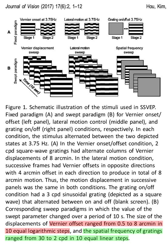
���Ѥ����f�H���B��ı/���ʲ��_�O��������������A�|�N����]���ݦ��V���ΦV�k���ʪ��]���A�äo���ʲ��_(optokinetic nystagmus)�C�����]�����O(grating acuity)��O����]���M�����G�ת��ťյe������X�{(grating onset/offset)(����)�C�o�˪��ܡA�ť߸����R���ӭn���R���W(
In patients with congenital esotropia, the kinesthetic/optico-nystagmus is asymmetrical on the nasotemporal
side, causing them to perceive inverted grating lines as moving to the left or
right, thus triggering optokinetic nystagmus. Grazing acuity is then achieved
by alternating between grating lines and blank areas of average brightness
(grating onset/offset) (see figure). Therefore, Fourier analysis should analyze
the fundamental frequency (1f) instead of its second harmonic (2f).
PowerDiva 1980�~�N���쫬�O�g�bApple-II�q���W���A�~���H�w�g�S�k�Q�����O�h���l���q���F�A�O����(RAM)�u��64KB�I�b�����}�x�����ҤU�A�o�a���W���{���N�Ӹɨ��C�O�o���j�Ʊб�����ɤ]�bTony������dz]�p�{���A�]�k��i���o�q�����H�����t�שM�IJv�C
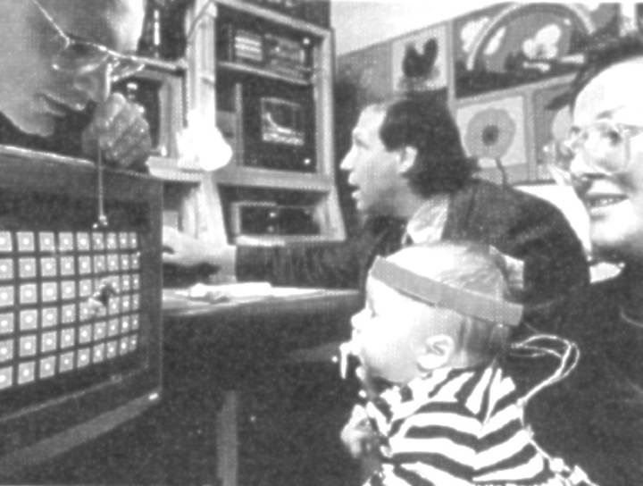
10���O�����e�A�q�`���X�������m�A��(adaptation)�e���A���ժ̽T�w����M�`�O�Ө�ù��W�F�A�~���s�Ұʥ���������E�����e���C
�Y�K�u�ݭn10�����`���ù��A�\�h�����٬O�S�k�@�������C���ժ̵o�{�L�����u���}�ù��ɡA�ߧY���s�Ȱ��O�����i�F���N�L���`�N�O�l�ަ^�ù�����A�A���s�}�l�O���C���Ҫ��O���|���Ƴ����Ȱ��e������E�A����N�X�q���i����B�s���_�ӡA�o�쥿�n10���������i�i����R�C(���ϡA�A�ݤ@����������o�q�쪺�ˬd�e��)
The PowerDiva prototype from the 1980s
was programmed into an Apple II computer�Xa very primitive computer for modern
people to imagine, with only 64KB of RAM! In such a challenging environment,
advanced programming technology was needed to compensate. I remember Tang Yu,
an associate professor at Zhejiang University, was designing programs in Tony's
lab at the time, trying to improve the speed and efficiency of evoked potential
signal extraction.
Before the 10-second recording, there were usually a few seconds
of adaptation screen. The tester confirmed that the child's attention was on
the screen before pressing the button to start the formal visual stimulus
sweep.
Even though only 10 seconds of screen focus was required, many
children couldn't complete it in one go. When the tester noticed the child's
gaze leave the screen, they immediately paused the
brainwave recording; after drawing the child's attention back to the screen,
they resumed recording. The restarted recording repeated parts of the visual
stimulus before the pause, and then the brainwave segments were trimmed and
connected to obtain exactly 10 seconds of brainwave data for analysis. (See the
image; view the examination footage of visual evoked potentials
in young children again.)

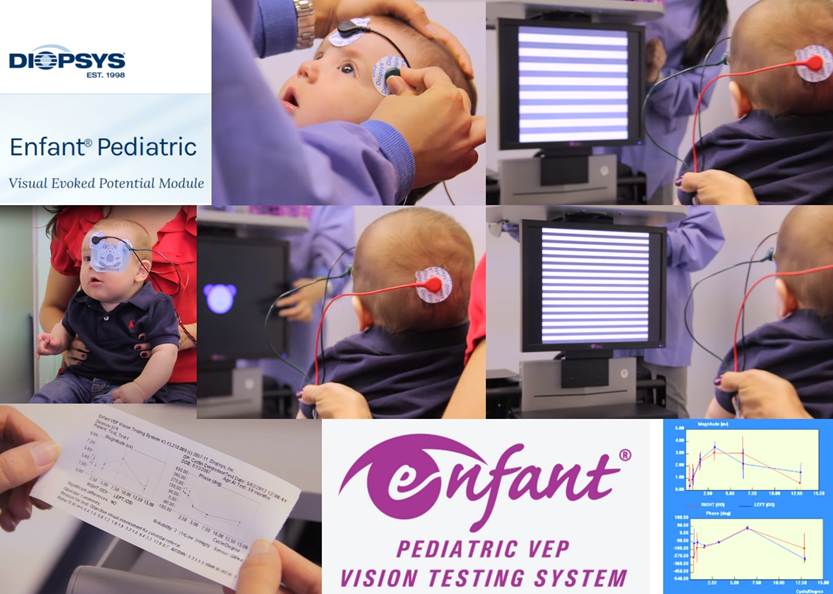
�ثePowerDiva�o�M�t�Φb����\�h��Ǥ��ߡB��ı��s���ߨϥΤ��C
�t�@�M�]�t���������o�q�쪺�t�Ϋh�ODiopsys
Enfant® Pediatric Visual Evoked Potential Module (����)
The PowerDiva system is currently used
in many medical centers and vision research centers in the United States.
Another system that includes grazing visual evoked potentials is the Diopsys Enfant®
Pediatric Visual Evoked Potential Module (see figure).
���q��(photocell)�@�������o�q�����Ǫ��ҫ��� �V ���ըt�Ϊ����T��
���e�s�@������䤣��F�A�����W��ǧ��ƹϨӸѻ��C
�D��O�������q��(photoresistor)�A�k�bBNC�y�W�A�T�w�b���������C�����o�q��Ϊ����i��j��(amplifier)�q�`��j100,000���A���q�ު������W�h�q�Ӥj�A�ós�@�ӹq��(BNC terminator)�N��n�C
A photocell serves as the model eye in a visual evoked potential
(VAP) lab �V testing the system's correctness.
The original physical model is lost, so I'm using material
diagrams found online for explanation.
The main component is the photoresistor, soldered to a BNC
connector and fixed to the bottom of the film holder. The EEG amplifier used
for VEP typically amplifies by 100,000��; directly connecting the photocell
would result in too much voltage, so connecting a resistor (BNC terminator) is
just right.

�o�O�ڭ̥H���q���N�H���A���զۤv�}�o�����������o�q�쪺�q���{���P�t�ΡC���T(amplitude)�M�ۦ�(phase)���Q�������C
This is our computer program and system for testing our
self-developed swept visual evoked potentials, using phototubes instead of the
human eye. The amplitude and phase are both perfect.
�p�G�ۦ�}�o�h�J�����q��/�����o�q��(Multifocal
ERG/VEP)�q���t�ΡA�@�˥i�H�Υ��q���N�H���A���ը������t�άO�_���T�C
If a multifocal ERG/VEP computer system is developed in-house,
phototubes can be used to replace the human eye to test and detect whether the
system is correct.
���O �V �Ʀ�ť߸����R (Digital Fourier Analysis)
���W²�u��BASIC�y���{���G
��bh���I
���m���W(mth harmonic)
[�D�ֳt�ť߸��Ǵ�(Fast Fourier Transform, FFT)]
Postscript �V Digital Fourier
Analysis
A short BASIC program is
attached: Horizontal axis: h points Decimate by m harmonics
[Non-Fast Fourier Transform
(FFT)]
real = 0: imag = 0
FOR i
= 0 TO h - 1
real
= real + y(i) * COS(2 * pi * i
* m / h)
imag = imag + y(i) * SIN(2 * pi * i * m / h)
NEXT
amp = (real ^ 2 + imag ^ 2) ^ .5 / h * 2
IF real = 0 AND imag > 0 THEN
phase = .5 * pi
ELSEIF real = 0 AND imag < 0 THEN
phase = 1.5 * pi
ELSE
phase = ATN(imag / real)
IF
real < 0 THEN phase = phase + pi
IF
real > 0 AND imag < 0 THEN phase = phase + 2 *
pi
END IF
IF phase >= 2 * pi THEN
phase = phase - 2 * pi
phase = phase / pi